Why you need “number intuition”
The goal is to be able to do rough estimates (back-of-the-envelope estimation). To judge at the system design stage whether “this architecture can meet the requirements for traffic volume, response speed, and availability,” you need the ability to get an order-of-magnitude sense before detailed measurement.
For questions like “can a single DB handle the assumed QPS?” or “won’t the number of network round-trips exceed the latency requirement?”, whether you can answer with an on-the-spot estimate greatly changes the speed and precision of design discussions. In System Design Interview (by Alex Xu, Socym), this back-of-the-envelope estimation is covered before the individual design problems.
What matters is not exact calculation but hitting the “order of magnitude.” In this article, I organize three numbers that form the foundation for that: powers of two, Jeff Dean’s latency table, and availability downtime conversions.
Powers of two: instantly converting data volume
Let me start with the powers of two you often see. Roughly tabulating the correspondence looks like this.
| Power | Approximate value | Number of zeros | Capacity | Media reference point |
|---|---|---|---|---|
| 2^10 | about 1,000 | 3 | 1KB | about 300 characters of Japanese text |
| 2^20 | about 1 million | 6 | 1MB | 1 phone photo (after compression) |
| 2^30 | about 1 billion | 9 | 1GB | about 10 minutes of video (full HD) |
| 2^40 | about 1 trillion | 12 | 1TB | 1 external HDD |
| 2^50 | about 1 quadrillion | 15 | 1PB | all logs of a large-scale service |
The only approximation to memorize is “2^10 ≒ 10^3 (about 1,000).” Everything else can be derived by multiplication. 2^20 = 2^10 × 2^10 ≒ 10^6 (1 million), 2^30 ≒ 10^9 (1 billion), and so on. Strictly, 2^10 is 1,024, so there’s an error, but it’s precise enough for the purpose of hitting the order of magnitude.
With this table in your head, you can answer questions like these instantly.
- How many GB is holding 1 billion int64 (8-byte) IDs? → 8 bytes × 10^9 = 8GB. An amount that fits in memory
- What about a table with 10 million records of 1KB each? → 10^3 bytes × 10^7 = 10GB
One caveat: in text estimates, one character isn’t always one byte. In UTF-8, alphanumerics are 1 byte, but Japanese is 3 bytes per character. About 300 Japanese characters fit in 1KB, which is the basis for the table’s reference point.
A conversion example: estimating storage for image uploads
Next is a practical example using this table. The subject is “a service where 1,000 users each upload one phone photo per day. What are the storage capacity and cost after one year?”
The procedure is three steps: “align the units → calculate only the order of magnitude → drop the fractions.”
- Align the units. Taking one phone photo as about 3MB, per day it’s 1,000 users × 3MB = 3,000MB = 3GB
- Calculate only the order of magnitude. Setting one year to about 400 days, 3GB × 400 ≒ 1.2TB. Calculating seriously with 365 days gives about 1.1TB, so the order of magnitude is right
- Convert to cost. Amazon S3 (Tokyo region) is about 0.025 USD per GB per month, so 1TB is about 25 USD/month, roughly 4,000 yen
So you can judge “at this scale, even accumulating for a year is a few thousand yen a month. It’s not the stage to agonize over storage design.”
Conversely, if users become 100 times more, at 100,000 people, it’s 300GB per day, about 110TB per year, and storage costs about 2,750 USD/month (about 400,000 yen). Once you get here, design decisions like lifecycle rules that move old images to a cheaper storage tier, or compression and resizing at upload time, become justifiable with numbers.
Jeff Dean’s latency table: learning speed differences in your bones
This is a list, presented by Google’s Dr. Jeff Dean, of the time taken by typical computer operations. The figures are from 2010, and some have become outdated due to faster hardware, but they’re still valid for grasping the order-of-magnitude sense of how fast or slow each operation is.
| Computer operation | Time |
|---|---|
| L1 cache reference | 0.5ns |
| Branch misprediction | 5ns |
| L2 cache reference | 7ns |
| Mutex lock/unlock | 100ns |
| Main memory reference | 100ns |
| Compress 1KB with zip | 10,000ns = 10μs |
| Send 2KB over 1Gbps network | 20,000ns = 20μs |
| Read 1MB sequentially from memory | 250,000ns = 250μs |
| Round trip within the same datacenter | 500,000ns = 500μs |
| Disk seek | 10,000,000ns = 10ms |
| Read 1MB sequentially from network | 10,000,000ns = 10ms |
| Read 1MB sequentially from disk | 30,000,000ns = 30ms |
| Send a packet round trip California-Netherlands | 150,000,000ns = 150ms |
Note: ns = nanosecond (10^-9 s), μs = microsecond (10^-6 s), ms = millisecond (10^-3 s). Converting, 1ms = 1,000μs = 1,000,000ns.
Reference: Google Pro Tip: Use Back-Of-The-Envelope-Calculations To Choose The Best Design
The following figure visualizes the figures as of 2020.
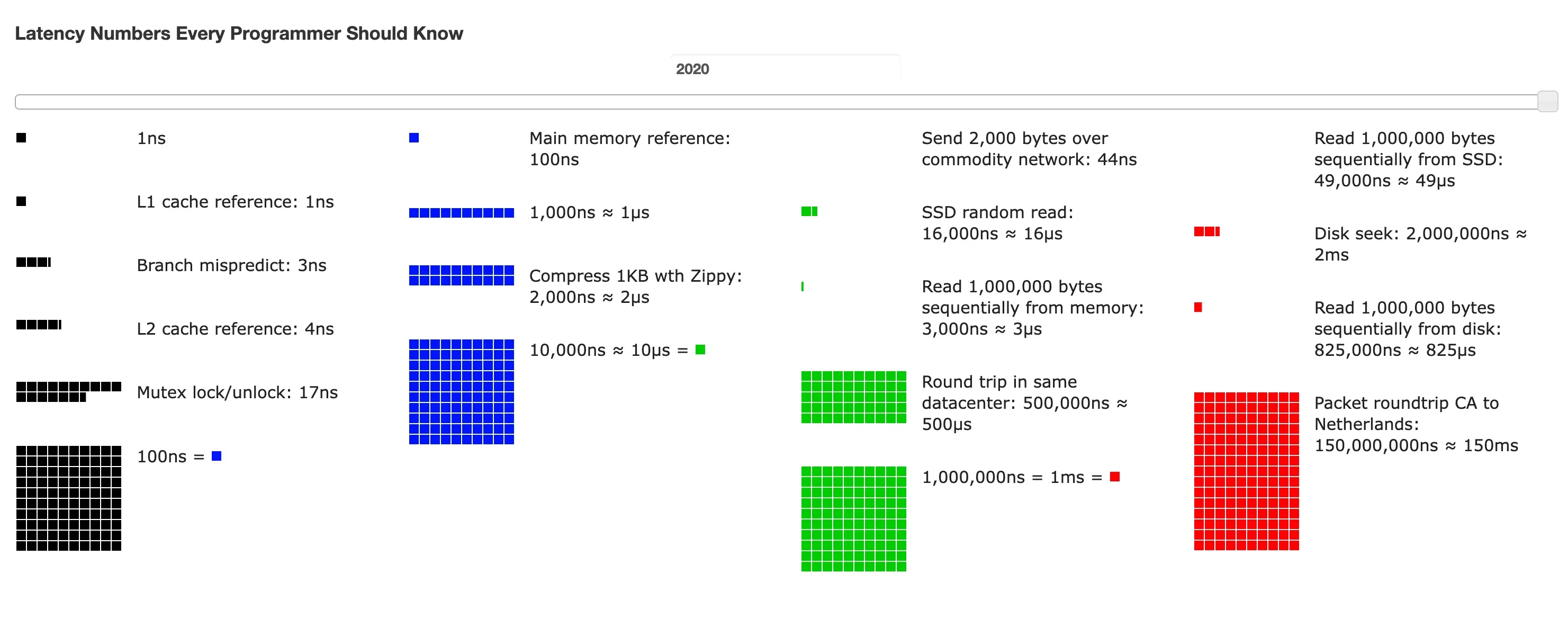
Source: Latency Numbers Every Programmer Should Know
Metrics usable in practice
From these figures, you can derive metrics usable directly in practical estimates.
- Sequential read from memory is about 4GB/s, SSD about 1GB/s, HDD about 30MB/s, and a 1Gbps network about 100MB/s
- In other words, memory is about 4 times faster than SSD and about 120 times faster than HDD
- A round trip within the same datacenter can be done about 2,000 times per second
- A global-scale round trip is limited to 6–7 times per second
- L2 cache is about 14 times slower than L1, and main memory about 200 times slower than L1
Reference: Latency Numbers Every Programmer Should Know
Design principles derivable from the table
This latency table serves as the “basis” for the design principles you use as a matter of course.
- Memory is overwhelmingly faster than disk. Comparing a 1MB sequential read, memory’s 250μs versus disk’s 30ms is a difference of over 100 times. This is why simply inserting a cache like Redis or Memcached changes the order of magnitude
- Avoid disk seeks (10ms). Reading and writing sequentially is faster than repeating random access. The reason append-only log designs like Kafka are fast is that they exploit this property
- Network round-trips become dominant. Even within a datacenter one round-trip takes 500μs, so an implementation with an increasing number of round-trips, like N+1 queries, is fatal in total even if each one is light. Across continents one round-trip is 150ms, so reducing round-trips and CDN/region placement connect directly to the latency requirement
- Compression is cheap. Compressing 1KB with zip is 10μs, a much lighter operation than network transfer. Compressing before transfer is basically a win because of this difference
The availability boundary: 99.9% is “1.44 minutes a day”
What’s often used when discussing availability is the SLA (Service Level Agreement). It’s a contract between a service provider and a customer that formally defines what level of uptime the service achieves. Uptime is traditionally measured in “the number of nines,” and more nines is considered better. Converting the allowed downtime per number of nines gives this.
| Availability (%) | Downtime per day | Downtime per week | Downtime per month | Downtime per year |
|---|---|---|---|---|
| 99% | 14.40 min | 1.68 hr | 7.31 hr | 3.65 days |
| 99.9% | 1.44 min | 10.08 min | 43.83 min | 8.77 hr |
| 99.99% | 8.64 sec | 1.01 min | 4.38 min | 52.60 min |
| 99.999% | 864.00 ms | 6.05 sec | 26.30 sec | 5.26 min |
| 99.9999% | 86.40 ms | 604.80 ms | 2.63 sec | 31.56 sec |
Points worth remembering.
- Major cloud providers like AWS, Google Cloud, and Microsoft Azure set their SLAs at 99.9% or higher
- Even at 99.9% (three nines), you can only be down 1.44 minutes per day. An operation that goes down for a few minutes on deploy or restart can violate the SLA just from that
- At 99.99% (four nines), it’s 8.64 seconds per day. That’s not a time a human can respond to manually; automatic failover becomes a prerequisite
- Each additional nine cuts the allowed downtime to one-tenth, and the cost to achieve it increases by an order of magnitude
Note that whereas an SLA is a contract with the customer, an internal team target is called an SLO (Service Level Objective). Google SRE also has the idea of treating the room until the SLO (the remaining allowed downtime) as an error budget, and releasing aggressively until it’s used up.
Availability drops multiplicatively as dependencies increase
Overall system availability is determined by the product of serially-dependent components.
Placing two services with 99.9% availability in series gives 0.999 × 0.999 ≒ 0.998, so the whole is 99.8%. The annual allowed downtime doubles from 8.77 hours to about 17.5 hours. If dependencies increase to 10, 0.999^10 ≒ 0.990, so even if each is three nines, the whole is 99%, dropping to a level of 3.65 days down per year. Increasing synchronous dependencies with microservices carries exactly this much cost in numerical terms.
Conversely, redundantly placing the same thing in parallel raises availability. With a configuration of two 99.9% servers in parallel where it’s fine if one is alive, it’s 1 - (1 - 0.999)^2 = 0.999999, so 99.9999%. Remembering “placing in series loses nines, and placing in parallel gains nines” lets you estimate the order of magnitude of availability just by looking at an architecture diagram.
Wrap-up
Finally, let me re-list the numbers to memorize from this article, narrowed to three.
- 2^10 ≒ 10^3. With just this one, you can derive everything up to 2^20 = 1 million (1MB) and 2^30 = 1 billion (1GB)
- The representative latency values. Memory is the world of μs, disk and inter-datacenter are the world of ms, and an inter-continental round trip is 150ms
- 99.9% is 1.44 minutes a day. Each additional nine cuts downtime to one-tenth and increases cost by an order of magnitude
With just this, storage estimates, the judgment of whether to insert a cache, and validity checks of an architecture against an SLA become doable by on-the-spot mental arithmetic. I think it’s fundamental knowledge that pays off in daily design reviews and the initial response to incidents.
References
 https://www.socym.co.jp/book/1406

https://medium.com/@bojanskr/latency-numbers-every-programmer-should-know-d85f8d3f8e6a